

Benchmarks#
Speed and region discovery of PSP() in psp-torch against the R package, and when the GPU is worth using, on two machines.
The R package’s benchmarks article measured psp 1.0.6 against 1.0.5. This notebook uses the same workloads and the same scripts to measure the R package against the PyTorch port, both run on one machine (a Windows PC with an Intel Xeon w5-2455X, 12 cores, 32 GB of memory and an NVIDIA T400), adds a study of CPU against GPU, and repeats the port’s side on a second machine (a Linux PC with an AMD Ryzen 7 5800X, 8 cores, 32 GB and an NVIDIA RTX 3060). Each build is named after what it ran on: the CPU for R and the port’s cpu builds (on Xeon w5-2455X, on Ryzen 7 5800X), the card for its cuda builds (on T400, on RTX 3060). The results and the scripts that produced them are in benchmarks/: compare.py runs the R scripts and the torch scripts in turn, and devices.py times the models on every device.
Three things to keep in mind when reading the numbers:
The R package calls the model once per parameter set; the port calls it once per iteration with every proposal in one batch. For the toy models here that is the whole difference, because the models themselves cost next to nothing. The
rowwiserows show the port calling the model one parameter set at a time, as R does.Random numbers differ, so runs with the same seed take different paths. Workloads are compared by their median over seeds.
The R package ran on the first machine only. Speed-ups against R are like for like for the first machine’s builds; for the second machine’s they also contain the difference between the two machines, which the port’s own builds on both show (the Ryzen 7 5800X runs four of the five toy workloads 1.3 to 1.8 times as fast as the Xeon w5-2455X, and the 1,000-region one a little slower).
The two cards are far apart. The T400 is a small card with 4 GB, the RTX 3060 a mid-range one with 12 GB and many times the cores and memory bandwidth; both, like most consumer cards, are slow in double precision. The device study measures float32 and float64 separately, on each machine.
from pathlib import Path
import numpy as np
import pandas as pd
import torch
from IPython.display import Markdown, display
import matplotlib.pyplot as plt
from matplotlib import patches as mpatches
from matplotlib.lines import Line2D
from figure_style import figures, titled

show = figures("benchmarks")

blue, grey = "#2a78d6", "#adb5bd"

# The first machine ran everything, R included; builds measured on another machine carry its name
# in parentheses (`--machine` of the benchmark scripts). In the figures and tables each build is named
# after what it ran on: the CPU for R and the cpu builds, the card for the cuda builds.
first_machine = "Xeon w5-2455X, T400"
other_machines = ["5800X, RTX 3060"]
machines = [first_machine, *other_machines]
hardware = {
    "Xeon w5-2455X, T400": {"cpu": "Xeon w5-2455X", "cuda": "T400"},
    "5800X, RTX 3060": {"cpu": "Ryzen 7 5800X", "cuda": "RTX 3060"},
}


def label(build):
    """`psp-torch 0.1.0 cuda (5800X, RTX 3060)` -> `psp-torch 0.1.0 cuda on RTX 3060`."""
    machine = next((m for m in other_machines if build.endswith(f" ({m})")), first_machine)
    base = build.removesuffix(f" ({machine})")
    return f"{base} on {hardware[machine]['cuda' if ' cuda' in base else 'cpu']}"


def machine_name(machine):
    return f"{hardware[machine]['cpu']} + {hardware[machine]['cuda']}"


def machine_of(build):
    return next(m for m in machines if build.split(" on ")[-1] in hardware[m].values())


def setup(build):
    """The build without where it ran: `psp-torch 0.1.0 cpu float64`."""
    return build.split(" on ")[0]


results = Path("../benchmarks/results")


def read(name):
    d = pd.read_csv(results / f"{name}.csv")
    return d.assign(build=d.build.map(label)) if "build" in d else d


workloads = read("workloads")
builds = list(dict.fromkeys(workloads.build))
r_build = next(b for b in builds if not b.startswith("psp-torch"))
torch_builds = [b for b in builds if b.startswith("psp-torch")]
palette = ["#6c757d", "#2a78d6", "#eb6834", "#1baf7a", "#eda100", "#4a3aa7", "#e34f8c", "#3fb5c4", "#8a6d3b"]
build_colours = dict(zip(builds, palette))
build_markers = dict(zip(builds, "osD^vP*Xh"))
Time per run#
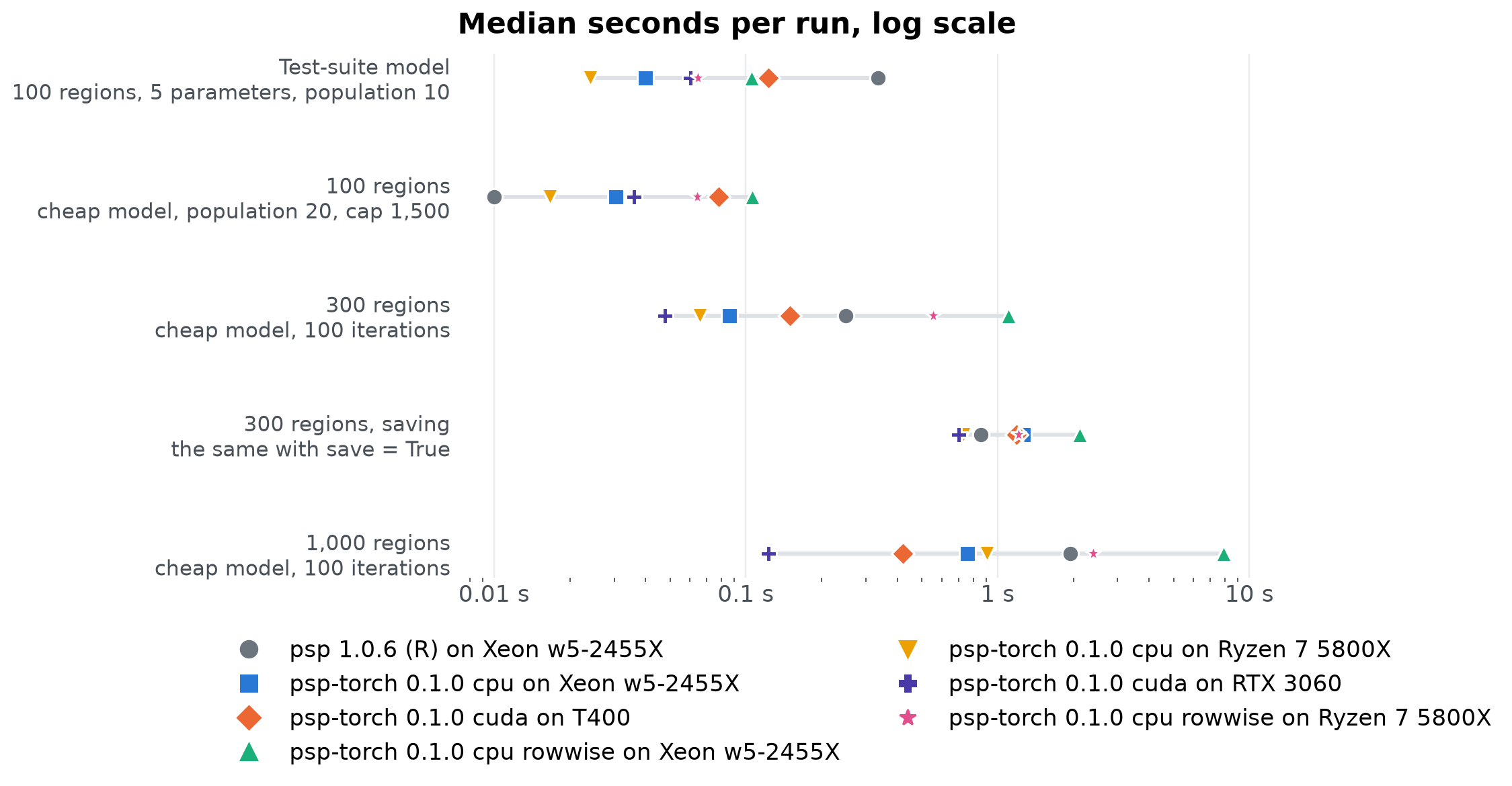
Each workload ran 3 to 10 times with different seeds; dots show the median wall-clock time of one complete PSP() run. The speed-up columns divide R’s time on the first machine by each build’s. The cheap toy models make each package’s own overhead visible: with the test-suite model, most of the time is the model itself.
order = list(dict.fromkeys(workloads.workload))
details = {
    "test model, pop 10": ("Test-suite model", "100 regions, 5 parameters, population 10"),
    "100 regions, pop 20, cap 1500": ("100 regions", "cheap model, population 20, cap 1,500"),
    "300 regions, 100 iterations": ("300 regions", "cheap model, 100 iterations"),
    "300 regions, 100 iterations, save": ("300 regions, saving", "the same with save = True"),
    "1000 regions, 100 iterations": ("1,000 regions", "cheap model, 100 iterations"),
}
median = workloads.groupby(["workload", "build"]).seconds.median().unstack()[builds].loc[order]
fig, ax = plt.subplots(figsize=(7, 4.6))
ys = np.arange(len(order))[::-1]
for y, w in zip(ys, order):
    row = median.loc[w]
    ax.plot([row.min(), row.max()], [y, y], color="#dee2e6", linewidth=2, zorder=1)
    for b in builds:
        ax.plot(row[b], y, build_markers[b], markersize=8, color=build_colours[b], markeredgecolor="white", zorder=2)
ax.set_xscale("log")
ax.set_yticks(ys, [f"{details[w][0]}\n{details[w][1]}" for w in order], fontsize=10)
ax.xaxis.set_major_formatter(lambda v, _: f"{v:g} s")
ax.grid(axis="y", visible=False)
handles = [Line2D([], [], marker=build_markers[b], linestyle="", markersize=8, color=build_colours[b], label=b)
           for b in builds]
ax.legend(handles=handles, loc="upper center", bbox_to_anchor=(0.5, -0.08), ncol=2)
titled(ax, "Median seconds per run, log scale")
show(fig, "workloads")
table = median.copy()
for b in torch_builds:
    table[f"speed-up, {b.replace('psp-torch 0.1.0 ', '')}"] = (median[r_build] / median[b]).map(lambda x: f"{x:.1f}×")
table.index = [details[w][0] for w in order]
table.round(3)
| build | psp 1.0.6 (R) on Xeon w5-2455X | psp-torch 0.1.0 cpu on Xeon w5-2455X | psp-torch 0.1.0 cuda on T400 | psp-torch 0.1.0 cpu rowwise on Xeon w5-2455X | psp-torch 0.1.0 cpu on Ryzen 7 5800X | psp-torch 0.1.0 cuda on RTX 3060 | psp-torch 0.1.0 cpu rowwise on Ryzen 7 5800X | speed-up, cpu on Xeon w5-2455X | speed-up, cuda on T400 | speed-up, cpu rowwise on Xeon w5-2455X | speed-up, cpu on Ryzen 7 5800X | speed-up, cuda on RTX 3060 | speed-up, cpu rowwise on Ryzen 7 5800X |
|---|---|---|---|---|---|---|---|---|---|---|---|---|---|
| Test-suite model | 0.335 | 0.040 | 0.123 | 0.105 | 0.024 | 0.060 | 0.065 | 8.4× | 2.7× | 3.2× | 13.9× | 5.6× | 5.2× |
| 100 regions | 0.010 | 0.030 | 0.078 | 0.106 | 0.017 | 0.036 | 0.064 | 0.3× | 0.1× | 0.1× | 0.6× | 0.3× | 0.2× |
| 300 regions | 0.250 | 0.086 | 0.150 | 1.104 | 0.066 | 0.048 | 0.556 | 2.9× | 1.7× | 0.2× | 3.8× | 5.3× | 0.4× |
| 300 regions, saving | 0.860 | 1.268 | 1.190 | 2.117 | 0.733 | 0.699 | 1.211 | 0.7× | 0.7× | 0.4× | 1.2× | 1.2× | 0.7× |
| 1,000 regions | 1.950 | 0.759 | 0.422 | 7.896 | 0.906 | 0.123 | 2.397 | 2.6× | 4.6× | 0.2× | 2.2× | 15.9× | 0.8× |
These are whole runs: the time from calling PSP() to getting its result back, including every model evaluation. They are short because the workloads are small and the models cost microseconds. Per workload, the median number of iterations and evaluations a run took, and what that makes one evaluation cost in each build:
size = workloads.groupby(["workload", "build"]).agg(iterations=("iterations", "median"), evaluations=("evaluations", "median"), seconds=("seconds", "median"))
per_evaluation = (1e6 * size.seconds / size.evaluations).unstack()[builds].loc[order]
context = pd.DataFrame({
    "Median iterations": size.iterations.unstack()[r_build].loc[order].map(lambda v: f"{v:,.0f}"),
    "Median evaluations": size.evaluations.unstack()[r_build].loc[order].map(lambda v: f"{v:,.0f}"),
    **{f"µs per evaluation, {b}": per_evaluation[b].round(1) for b in builds},
})
context.index = [details[w][0] for w in order]
context
| Median iterations | Median evaluations | µs per evaluation, psp 1.0.6 (R) on Xeon w5-2455X | µs per evaluation, psp-torch 0.1.0 cpu on Xeon w5-2455X | µs per evaluation, psp-torch 0.1.0 cuda on T400 | µs per evaluation, psp-torch 0.1.0 cpu rowwise on Xeon w5-2455X | µs per evaluation, psp-torch 0.1.0 cpu on Ryzen 7 5800X | µs per evaluation, psp-torch 0.1.0 cuda on RTX 3060 | µs per evaluation, psp-torch 0.1.0 cpu rowwise on Ryzen 7 5800X | |
|---|---|---|---|---|---|---|---|---|---|
| Test-suite model | 136 | 1,756 | 190.7 | 21.8 | 67.7 | 57.4 | 13.1 | 33.1 | 35.2 |
| 100 regions | 78 | 2,235 | 4.5 | 13.6 | 35.1 | 47.4 | 7.5 | 16.2 | 28.6 |
| 300 regions | 100 | 24,202 | 10.3 | 3.6 | 6.2 | 46.7 | 2.8 | 2.0 | 23.5 |
| 300 regions, saving | 100 | 24,202 | 35.5 | 53.6 | 49.5 | 89.6 | 31.0 | 29.1 | 51.2 |
| 1,000 regions | 100 | 82,098 | 23.8 | 9.3 | 5.2 | 96.6 | 11.1 | 1.5 | 29.3 |
To see one for yourself, this cell runs the 100-region workload once, here and now, and times the whole call:
import time

from psp import PSP
from psp.models.voronoi import voronoi_control, voronoi_model

v = voronoi_model(100, 5)
generator = torch.Generator().manual_seed(1)
start = time.perf_counter()
result = PSP(v.model, v.discretize, voronoi_control(100, 5, 1500, 20), quiet=True, generator=generator)
elapsed = time.perf_counter() - start
print(f"{elapsed:.3f} s for the whole run: {result.iterations} iterations, {result.evaluations:,} evaluations, "
      f"{result.patterns} regions, {1e6 * elapsed / result.evaluations:.1f} µs per evaluation")
0.019 s for the whole run: 100 iterations, 2,200 evaluations, 95 regions, 8.8 µs per evaluation
On the 100-region workload, the R package filled every region in 5 of 5 runs after a median of 2,235 model evaluations; the port on the CPU of the same machine filled them in 5 of 5 runs after a median of 2,241. The samplers are the same algorithm, so the evaluations they need are alike; the time differs because of what each does around them. That workload is also the one place the R package wins: about 78 iterations of a few microseconds each, a run so short that per-iteration overhead is all there is, and R’s own timer only resolves it to 10 ms. The port’s cost per iteration is higher (a few hundred microseconds of Python and tensor dispatch) and its cost per evaluation lower, so it pulls ahead as soon as iterations carry more than a handful of parameter sets.
Where the time goes#
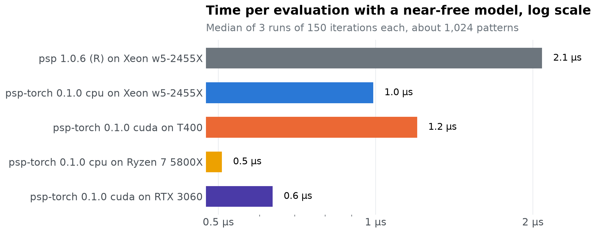
To isolate each package’s own cost, this test uses a model that does almost nothing: it returns its parameters, and discretize bins them into 1,024 grid cells. The R script times those two functions from a plain R loop and subtracts; the torch script times them one parameter set at a time (callbacks_us, the R way) and in one batch per iteration (batched_us, the way PSP() calls them).
overhead = read("overhead")
summary = overhead.groupby("build").median(numeric_only=True)
summary = summary.loc[[b for b in builds if b in summary.index]]
fig, ax = plt.subplots(figsize=(7, 1 + 0.5 * len(summary)))
ys = np.arange(len(summary))[::-1]
ax.barh(ys, summary.total_us, color=[build_colours[b] for b in summary.index], height=0.6)
for y, (b, row) in zip(ys, summary.iterrows()):
    ax.text(row.total_us * 1.05, y, f"{row.total_us:.1f} µs", va="center", fontsize=10.5)
ax.set_xscale("log")
ax.set_yticks(ys, summary.index)
ax.xaxis.set_major_formatter(lambda v, _: f"{v:g} µs")
ax.xaxis.set_minor_formatter(plt.NullFormatter())
ticks = [t for t in (0.1, 0.2, 0.5, 1, 2, 5, 10, 20, 50, 100)
         if summary.total_us.min() / 1.5 <= t <= summary.total_us.max() * 1.5]
ax.set_xticks(ticks, [f"{t:g} µs" for t in ticks])
ax.grid(axis="y", visible=False)
titled(ax, "Time per evaluation with a near-free model, log scale",
       f"Median of 3 runs of 150 iterations each, about {summary.patterns.iloc[0]:,.0f} patterns")
show(fig, "overhead")
cols = [c for c in ["evaluations", "patterns", "total_us", "callbacks_us", "batched_us", "framework_us"] if c in summary]
summary[cols].round(2)
| evaluations | patterns | total_us | callbacks_us | batched_us | framework_us | |
|---|---|---|---|---|---|---|
| build | ||||||
| psp 1.0.6 (R) on Xeon w5-2455X | 134468.0 | 1024.0 | 2.08 | 2.01 | NaN | 0.07 |
| psp-torch 0.1.0 cpu on Xeon w5-2455X | 134724.0 | 1024.0 | 0.99 | 16.24 | 0.01 | -15.37 |
| psp-torch 0.1.0 cuda on T400 | 136324.0 | 1024.0 | 1.20 | 62.60 | 0.03 | -61.44 |
| psp-torch 0.1.0 cpu on Ryzen 7 5800X | 134724.0 | 1024.0 | 0.51 | 9.72 | 0.02 | -9.22 |
| psp-torch 0.1.0 cuda on RTX 3060 | 136324.0 | 1024.0 | 0.64 | 28.80 | 0.00 | -28.13 |
framework_us is the time per evaluation that is not spent in the two callbacks called one at a time: for R, the package’s own bookkeeping; for the port, it is negative, because batching the callbacks saves more than the sampler costs. The port’s own cost per iteration is a few hundred microseconds whatever the batch size, so with many patterns filling at once it is spread thin, and with one or two it dominates.
Saving to disk#
With save=True, every evaluation writes its parameters and its model outputs, here 300 values, to csv. Both packages write full precision: the R package the shortest text that reads back as the same double (with std::to_chars), the port the same through Python’s repr.
save = read("save").groupby("build").median(numeric_only=True)
save = save.loc[[b for b in builds if b in save.index]]
save[["evaluations", "save_us", "total_us", "mb"]].round(1)
| evaluations | save_us | total_us | mb | |
|---|---|---|---|---|
| build | ||||
| psp 1.0.6 (R) on Xeon w5-2455X | 24202.0 | 25.3 | 34.9 | 140.3 |
| psp-torch 0.1.0 cpu on Xeon w5-2455X | 23640.0 | 47.3 | 51.7 | 137.0 |
| psp-torch 0.1.0 cuda on T400 | 24035.0 | 43.6 | 48.8 | 139.3 |
| psp-torch 0.1.0 cpu on Ryzen 7 5800X | 23640.0 | 29.4 | 31.0 | 137.0 |
| psp-torch 0.1.0 cuda on RTX 3060 | 24035.0 | 27.2 | 29.2 | 139.3 |
Finding regions#
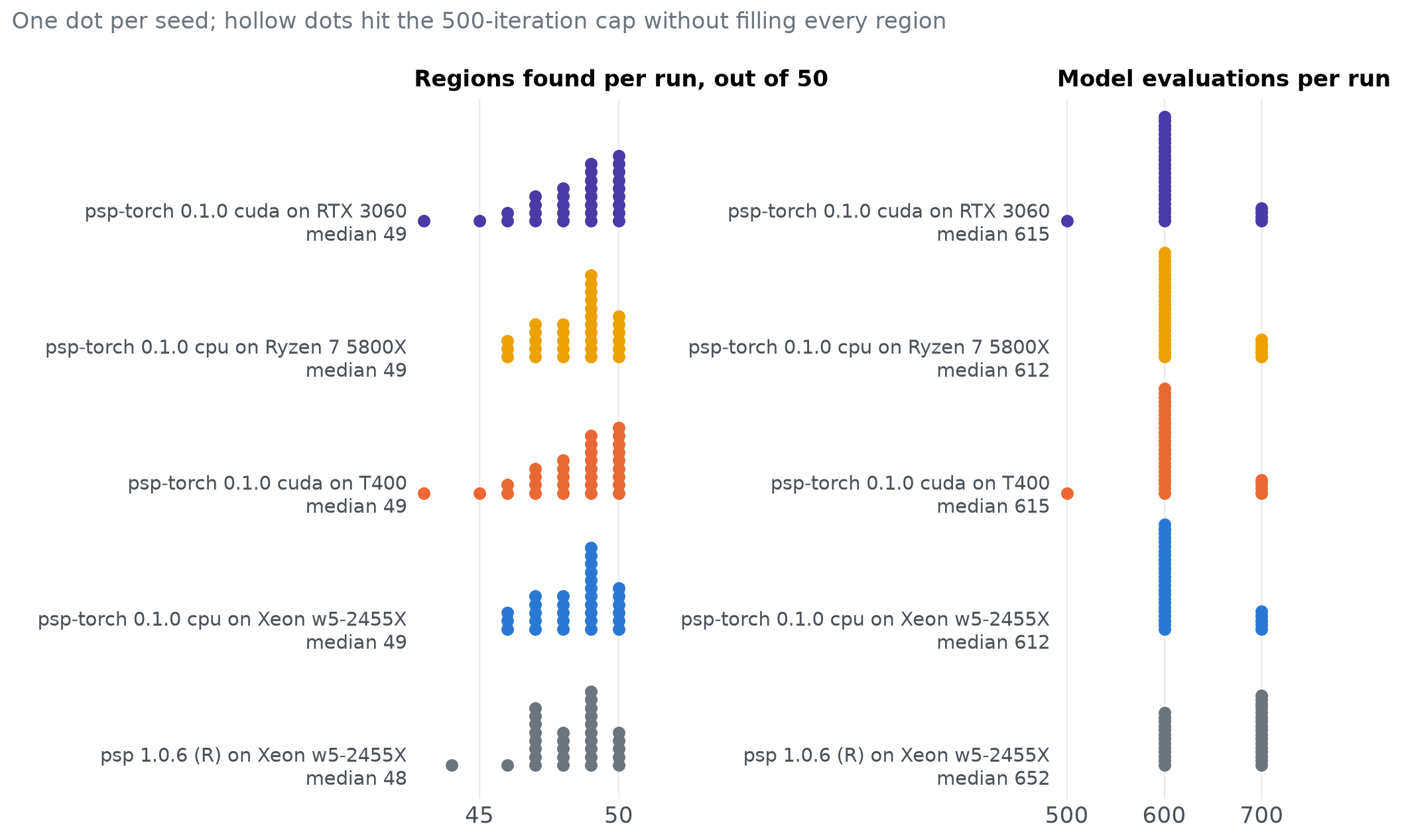
Faster is only useful if the search still finds the regions. These are 30 runs per build on a 50-region model with 3 parameters, population 10, radius 0.3 and a 500-iteration cap. The samplers are the same algorithm with different random numbers, so they should find about the same number of regions with about the same number of evaluations.
discovery = read("discovery")
discovery["filled"] = discovery.filled.astype(str).str.lower().isin(["true", "1"])
present = [b for b in builds if b in set(discovery.build)]
fig, axes = plt.subplots(1, 2, figsize=(9, 1.4 + 0.9 * len(present)))
for ax, key, title in zip(axes, ["regions", "evaluations"], ["Regions found per run, out of 50", "Model evaluations per run"]):
    binned = [discovery[discovery.build == b][key] if key == "regions"
              else (discovery[discovery.build == b][key] / 100).round() * 100 for b in present]
    step = min(0.12, 1.6 / max(v.value_counts().max() for v in binned))  # the tallest stack fills 1.6 rows
    for i, b in enumerate(present):
        d = discovery[discovery.build == b]
        values = d[key] if key == "regions" else (d[key] / 100).round() * 100
        stacks = {}
        for v, filled in zip(values, d.filled):
            n = stacks.get(v, 0); stacks[v] = n + 1
            ax.plot(v, 2 * i + step * n, "o", markersize=5, color=build_colours[b] if filled else "white",
                    markeredgecolor=build_colours[b], markeredgewidth=1.2)
    ax.set_yticks([2 * i for i in range(len(present))], [f"{b}\nmedian {discovery[discovery.build == b][key].median():,.0f}" for b in present], fontsize=9.5)
    ax.set_ylim(-0.5, 2 * len(present) - 0.2)
    ax.grid(axis="y", visible=False)
    ax.set_title(title, loc="left", fontsize=11)
axes[1].xaxis.set_major_formatter(lambda v, _: f"{v:,.0f}")
fig.suptitle("One dot per seed; hollow dots hit the 500-iteration cap without filling every region", x=0.02, ha="left",
             fontsize=11, color="#6c757d", fontweight="normal")
fig.tight_layout()
show(fig, "discovery")
discovery.groupby("build").agg(runs=("seed", "size"), regions=("regions", "median"), evaluations=("evaluations", "median"),
                               filled=("filled", "sum")).loc[present]
| runs | regions | evaluations | filled | |
|---|---|---|---|---|
| build | ||||
| psp 1.0.6 (R) on Xeon w5-2455X | 30 | 48.5 | 652.0 | 30 |
| psp-torch 0.1.0 cpu on Xeon w5-2455X | 30 | 49.0 | 611.5 | 30 |
| psp-torch 0.1.0 cuda on T400 | 30 | 49.0 | 615.0 | 30 |
| psp-torch 0.1.0 cpu on Ryzen 7 5800X | 30 | 49.0 | 611.5 | 30 |
| psp-torch 0.1.0 cuda on RTX 3060 | 30 | 49.0 | 615.0 | 30 |
PSP never guarantees finding every region. It only finds regions it can reach before every found region is full. The settings below change that, measured on the same model with 30 seeds each:
settings = read("settings")
settings["filled"] = settings.filled.astype(str).str.lower().isin(["true", "1"])
settings = settings[settings.build == cpu_build]
order = list(dict.fromkeys(settings.setting))
table = settings.groupby("setting").agg(
    lo=("regions", "min"), hi=("regions", "max"), median=("regions", "median"),
    all_50=("regions", lambda r: int((r == 50).sum())), runs=("seed", "size"), evaluations=("evaluations", "median"),
).loc[order]
pd.DataFrame({
    "Settings": order,
    "Regions found per run": [f"{int(r.lo)}–{int(r.hi)}, median {r['median']:.0f}" for _, r in table.iterrows()],
    "Runs that found all 50": [f"{int(r.all_50)} of {int(r.runs)}" for _, r in table.iterrows()],
    "Median evaluations": [f"{r.evaluations:,.0f}" for _, r in table.iterrows()],
}).set_index("Settings")
| Regions found per run | Runs that found all 50 | Median evaluations | |
|---|---|---|---|
| Settings | |||
| 1 start, population 10, radius 0.3 | 46–50, median 49 | 6 of 30 | 612 |
| 10 random starts, population 10 | 43–50, median 49 | 10 of 30 | 620 |
| 1 start, population 30 | 49–50, median 50 | 29 of 30 | 1,728 |
| 1 start, population 10, radius 0.5 | 49–50, median 50 | 26 of 30 | 726 |
| 10 random starts, population 30 | 50–50, median 50 | 30 of 30 | 1,750 |
| 3 pooled runs of 10 starts, population 10 | 50–50, median 50 | 30 of 30 | 1,862 |
Raising population helps most. A larger radius is cheaper, but in a real model it can jump over small regions. Pooling independent runs is a useful completeness check: if a second run finds a pattern the first missed, the first wasn’t complete. The tutorial shows how.
When is the GPU worth it?#
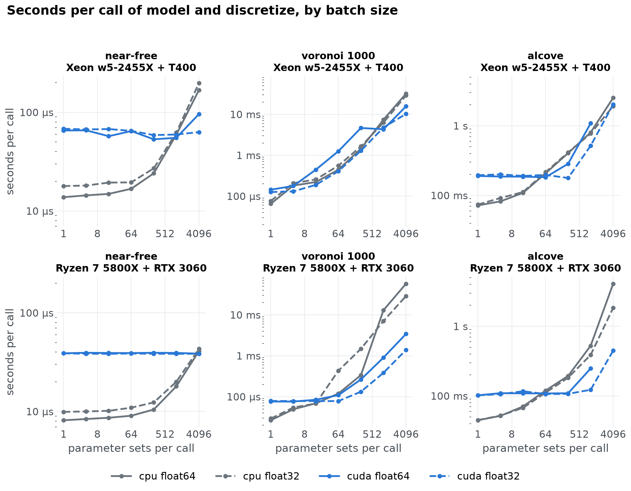
Two things decide whether a run gains from the GPU: how much work one call of model does, and how many parameter sets each call receives, which in a PSP run is the number of patterns still filling. devices.py measures both. First, model and discretize alone, for batches of 1 to 4,096 parameter sets, with three models: a near-free one (it returns its parameters), the Voronoi model with 1,000 centres (a (n, 1000) distance matrix per call), and ALCOVE with 30 simulated learners (256 sequential trials of a small network per call).
devices = read("devices")
calls = devices[devices.kind == "model"]
models = list(dict.fromkeys(calls.model))
device_machines = [m for m in machines if m in set(devices.machine)]
styles = {("cpu", "float64"): ("#6c757d", "-"), ("cpu", "float32"): ("#6c757d", "--"),
          ("cuda", "float64"): ("#2a78d6", "-"), ("cuda", "float32"): ("#2a78d6", "--")}
fig, grid = plt.subplots(len(device_machines), len(models), figsize=(10, 0.5 + 3.6 * len(device_machines)),
                         sharey="col", squeeze=False)
for row, machine in zip(grid, device_machines):
    for ax, m in zip(row, models):
        for (dev, dt), (colour, style) in styles.items():
            d = calls[(calls.machine == machine) & (calls.model == m) & (calls.device == dev) & (calls.dtype == dt)].sort_values("batch")
            if len(d):
                ax.plot(d.batch, d.seconds, style, color=colour, linewidth=2, marker="o", markersize=4, label=f"{dev} {dt}")
        ax.set_xscale("log", base=2); ax.set_yscale("log")
        ax.set_title(f"{m}\n{machine_name(machine)}", loc="center", fontsize=11)
        ax.xaxis.set_major_formatter(lambda v, _: f"{v:g}")
        ax.yaxis.set_major_formatter(lambda v, _: f"{v:g} s" if v >= 1 else f"{v * 1000:g} ms" if v >= 1e-3 else f"{v * 1e6:g} µs")
    row[0].set_ylabel("seconds per call")
for ax in grid[-1]:
    ax.set_xlabel("parameter sets per call")
fig.legend(*grid[0, 0].get_legend_handles_labels(), loc="lower center", ncol=4, bbox_to_anchor=(0.5, 0))
fig.suptitle("Seconds per call of model and discretize, by batch size", x=0.02, ha="left", fontweight="bold")
fig.tight_layout(rect=(0, 0.05, 1, 0.96))
show(fig, "devices")
def call_times(machine, m, dev, dt):
    return calls[(calls.machine == machine) & (calls.model == m) & (calls.device == dev) & (calls.dtype == dt)].set_index("batch").seconds


rows = []
for machine in device_machines:
    for m in models:
        for dt in ("float32", "float64"):
            cpu, gpu = call_times(machine, m, "cpu", dt), call_times(machine, m, "cuda", dt)
            if len(gpu) == 0:
                continue
            common = cpu.index.intersection(gpu.index)
            faster = [b for b in common if gpu[b] < cpu[b]]
            rows.append({"machine": machine_name(machine), "model": m, "dtype": dt, "GPU faster from batch": min(faster) if faster else "never",
                         "speed-up at largest batch": f"{cpu[common.max()] / gpu[common.max()]:.1f}×"})
crossover = pd.DataFrame(rows).set_index(["machine", "model", "dtype"])
crossover
| GPU faster from batch | speed-up at largest batch | |||
|---|---|---|---|---|
| machine | model | dtype | ||
| Xeon w5-2455X + T400 | near-free | float32 | 1024 | 3.1× |
| float64 | 1024 | 1.8× | ||
| voronoi 1000 | float32 | 4 | 2.8× | |
| float64 | 4 | 2.0× | ||
| alcove | float32 | 64 | 0.9× | |
| float64 | 64 | 0.7× | ||
| Ryzen 7 5800X + RTX 3060 | near-free | float32 | 4096 | 1.1× |
| float64 | 4096 | 1.1× | ||
| voronoi 1000 | float32 | 64 | 20.7× | |
| float64 | 64 | 16.8× | ||
| alcove | float32 | 64 | 4.1× | |
| float64 | 64 | 2.1× |
Then whole runs of PSP() on the same models. The batch size of a run is set here by the number of starting points, with a population that keeps every pattern filling, so the search proposes about as many parameter sets per iteration as it has starts:
runs = devices[devices.kind == "psp"].copy()
runs["per_evaluation_us"] = 1e6 * runs.seconds / runs.evaluations
pivot = runs.pivot_table(index=["model", "batch"], columns=["machine", "device", "dtype"], values="seconds")[device_machines].rename(columns=machine_name, level="machine")
pivot.round(3)
| machine | Xeon w5-2455X + T400 | Ryzen 7 5800X + RTX 3060 | |||||||
|---|---|---|---|---|---|---|---|---|---|
| device | cpu | cuda | cpu | cuda | |||||
| dtype | float32 | float64 | float32 | float64 | float32 | float64 | float32 | float64 | |
| model | batch | ||||||||
| alcove | 1 | 1.712 | 1.642 | 3.776 | 3.880 | 1.123 | 1.292 | 2.163 | 2.221 |
| 16 | 2.351 | 2.376 | 3.932 | 4.068 | 1.350 | 1.279 | 2.269 | 2.270 | |
| near-free | 1 | 0.009 | 0.010 | 0.037 | 0.038 | 0.007 | 0.006 | 0.018 | 0.018 |
| 16 | 0.015 | 0.016 | 0.041 | 0.043 | 0.010 | 0.010 | 0.022 | 0.022 | |
| 256 | 0.030 | 0.032 | 0.052 | 0.055 | 0.020 | 0.022 | 0.029 | 0.029 | |
| voronoi 1000 | 1 | 0.021 | 0.024 | 0.040 | 0.042 | 0.011 | 0.010 | 0.021 | 0.020 |
| 16 | 0.065 | 0.078 | 0.057 | 0.071 | 0.022 | 0.026 | 0.025 | 0.028 | |
| 256 | 0.257 | 0.302 | 0.112 | 0.191 | 0.128 | 0.392 | 0.039 | 0.056 | |
What the numbers say on the two machines:
near-free: the GPU is on the Xeon w5-2455X + T400 machine at best 3.1× the CPU in float32 (at 4,096 parameter sets per call) and 1.8× in float64 (at 4,096); on the Ryzen 7 5800X + RTX 3060 machine at best 1.1× the CPU in float32 (at 4,096 parameter sets per call) and 1.1× in float64 (at 4,096).
voronoi 1000: the GPU is on the Xeon w5-2455X + T400 machine at best 2.8× the CPU in float32 (at 4,096 parameter sets per call) and 2.0× in float64 (at 4,096); on the Ryzen 7 5800X + RTX 3060 machine at best 20.7× the CPU in float32 (at 4,096 parameter sets per call) and 16.8× in float64 (at 4,096).
alcove: the GPU is on the Xeon w5-2455X + T400 machine at best 2.3× the CPU in float32 (at 256 parameter sets per call) and 1.4× in float64 (at 256); on the Ryzen 7 5800X + RTX 3060 machine at best 4.1× the CPU in float32 (at 4,096 parameter sets per call) and 2.1× in float64 (at 1,024).
A model that costs microseconds never gains in a run. A single call of the near-free model does win once the batch is in the thousands, but a PSP run never proposes that many at once, and every iteration costs a handful of kernel launches and a copy of the patterns back to the CPU, about as much as a whole iteration costs on the CPU. Its runs are slower on the GPU at every batch size, on either card.
A model that does real tensor work per parameter set gains once each call carries enough of them, here from a handful of parameter sets on the T400 and a few dozen on the RTX 3060 (whose CPU is also faster) for the Voronoi model, which is one
(n, 1000)distance matrix per call. The gain grows with the batch, and with the card: the RTX 3060 has many times the T400’s cores and memory bandwidth, so at large batches its lead over its CPU is far larger than the T400’s.A sequential model gains less than its size suggests. ALCOVE is 256 small steps in a row; each step is a few kernels whatever the batch, so the GPU only pulls ahead once the batch is in the dozens to hundreds. On the T400 the gain peaks around 2× before the card itself becomes the limit; the RTX 3060 keeps gaining up to the largest batch. In float64 the gain is smaller on both: consumer cards run double precision at a small fraction of their float32 rate.
A PSP run is only as batched as its iterations. The batch is the number of patterns still filling: few at the start, more in the middle, and a few stubborn regions at the end. The ALCOVE runs above, with 1 and 16 starting points, propose too few parameter sets per iteration to gain (on the Xeon w5-2455X + T400 machine 2.4 s on the CPU against 3.9 s on the GPU in float32; on the Ryzen 7 5800X + RTX 3060 machine 1.3 s on the CPU against 2.3 s on the GPU in float32). A run gains when its middle is wide: many patterns, large populations, and a model that costs milliseconds per batch on the CPU.
So: start on the CPU, where the port already batches the model and beats the R package by the margins above. Move to the GPU when a single call of your model with the batch sizes your run actually produces is faster there (devices.py is a template for that measurement), use float32 if the model allows it, and expect a larger card to move every crossover to the left, as the RTX 3060 does against the T400.
ALCOVE on its full parameter space#
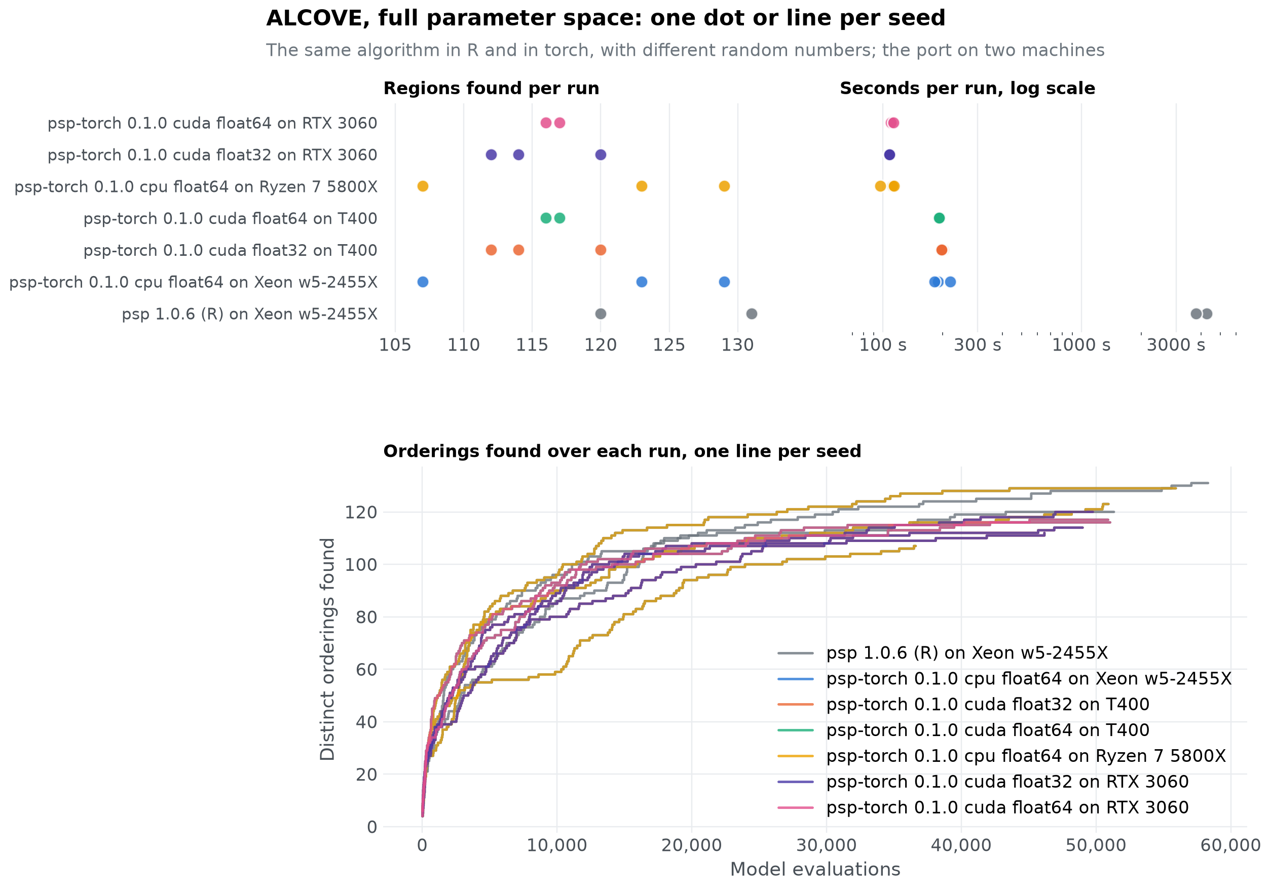
The workloads above use toy models. This one is the real thing: the ALCOVE recipe with the learning rates free over their full range (specificity 0 to 20, decision consistency 0 to 6, both learning rates 0 to 1, lower bounds just above 0 because ALCOVE rejects a learning rate of exactly 0), 20 random starting points, radius 0.15, population 50 and a cap of 1,000 iterations, with catlearn’s trial order for seed 7624 and 5 simulated learners per type. Each build ran it with seeds 1, 2 and 3. The port’s random numbers come from torch’s generators, which give the same stream on any machine, so a build run on both machines with the same seed takes the same path: the same evaluations, the same regions, only the time differs. In the curves below, the second machine’s lines lie on top of the first machine’s. Two runs are left out as outliers: R’s seed 1, which stopped after 397 iterations with 6 regions (its 20 starting points landed in 6 regions, no proposal from them reached another, and all 6 filled), and the port’s GPU float64 seed 2, which found 61 regions from 21,746 evaluations where every other run found over a hundred, on both machines. Both are the search itself getting stuck early, which the same settings produce on either side now and then; the tutorial shows how repeated runs guard against it. The R package calls catlearn’s slpALCOVE() once per parameter set; the port calls the batched ALCOVE once per iteration. Both save every evaluation, so the number of distinct orderings found can be followed iteration by iteration.
The scripts are benchmarks/alcove_benchmark.py and benchmarks/r/alcove_benchmark.R.
# the outliers of the text; those of the first machine were taken out of the csv files when it was measured
outliers = {("psp-torch 0.1.0 cuda float64 on RTX 3060", 2)}


def read_alcove(name):
    d = read(name)
    return d[[(b, s) not in outliers for b, s in zip(d.build, d.seed)]]


alcove = read_alcove("alcove")
alcove["filled"] = alcove.filled.astype(str).str.lower().isin(["true", "1"])
all_builds = list(dict.fromkeys(alcove.build))
alcove_builds = [b for b in all_builds if not b.startswith("psp-torch")] + [b for b in all_builds if b.startswith("psp-torch")]
alcove_colours = dict(zip(alcove_builds, palette))
table = alcove.groupby("build").agg(
    runs=("seed", "size"), seconds=("seconds", "median"),
    regions_min=("patterns", "min"), regions_median=("patterns", "median"), regions_max=("patterns", "max"),
    evaluations=("evaluations", "median"), iterations=("iterations", "median"), filled=("filled", "sum"),
).loc[alcove_builds]
found_all = read_alcove("alcove_patterns")
nan_patterns = found_all[found_all.order.isna()].groupby(["build", "seed"]).size()
nan_share = (found_all[found_all.order.isna()].groupby("build")["count"].sum()
             / found_all.groupby("build")["count"].sum()).reindex(alcove_builds).fillna(0)
pd.DataFrame({
    "Runs": table.runs.astype(int),
    "Median minutes per run": (table.seconds / 60).round(1),
    "Regions found per run": [f"{int(r.regions_min)}–{int(r.regions_max)}, median {r.regions_median:.0f}" for _, r in table.iterrows()],
    "Of which NaN patterns": [", ".join(str(int(nan_patterns.get((b, seed), 0))) for seed in sorted(alcove[alcove.build == b].seed.unique())) for b in alcove_builds],
    "Evaluations in NaN patterns": [f"{nan_share[b]:.1%}" for b in alcove_builds],
    "Median evaluations": table.evaluations.map(lambda v: f"{v:,.0f}"),
    "Median iterations": table.iterations.map(lambda v: f"{v:,.0f}"),
    "Runs that filled every region": [f"{int(r.filled)} of {int(r.runs)}" for _, r in table.iterrows()],
}, index=alcove_builds)
| Runs | Median minutes per run | Regions found per run | Of which NaN patterns | Evaluations in NaN patterns | Median evaluations | Median iterations | Runs that filled every region | |
|---|---|---|---|---|---|---|---|---|
| psp 1.0.6 (R) on Xeon w5-2455X | 2 | 67.3 | 120–131, median 126 | 16, 6 | 7.3% | 54,816 | 1,000 | 0 of 2 |
| psp-torch 0.1.0 cpu float64 on Xeon w5-2455X | 3 | 3.2 | 107–129, median 123 | 0, 0, 0 | 0.0% | 50,917 | 1,000 | 0 of 3 |
| psp-torch 0.1.0 cuda float32 on T400 | 3 | 3.3 | 112–120, median 114 | 0, 0, 0 | 0.0% | 49,002 | 1,000 | 0 of 3 |
| psp-torch 0.1.0 cuda float64 on T400 | 2 | 3.2 | 116–117, median 116 | 0, 0 | 0.0% | 50,968 | 1,000 | 0 of 2 |
| psp-torch 0.1.0 cpu float64 on Ryzen 7 5800X | 3 | 1.9 | 107–129, median 123 | 0, 0, 0 | 0.0% | 50,917 | 1,000 | 0 of 3 |
| psp-torch 0.1.0 cuda float32 on RTX 3060 | 3 | 1.8 | 112–120, median 114 | 0, 0, 0 | 0.0% | 49,002 | 1,000 | 0 of 3 |
| psp-torch 0.1.0 cuda float64 on RTX 3060 | 2 | 1.9 | 116–117, median 116 | 0, 0 | 0.0% | 50,968 | 1,000 | 0 of 2 |
curves = read_alcove("alcove_discovery")
fig = plt.figure(figsize=(10, 8.5))
grid = fig.add_gridspec(2, 2, height_ratios=[1, 1.6], hspace=0.45, wspace=0.12)
strips = [fig.add_subplot(grid[0, 0]), fig.add_subplot(grid[0, 1])]
for ax, key, title in zip(strips, ["patterns", "seconds"], ["Regions found per run", "Seconds per run, log scale"]):
    for i, b in enumerate(alcove_builds):
        d = alcove[alcove.build == b]
        ax.plot(d[key], [i] * len(d), "o", markersize=8, color=alcove_colours[b], markeredgecolor="white", alpha=0.85)
    ax.set_yticks(range(len(alcove_builds)), alcove_builds, fontsize=10)
    ax.set_ylim(-0.6, len(alcove_builds) - 0.4)
    ax.grid(axis="y", visible=False)
    ax.set_title(title, loc="left", fontsize=11)
strips[0].margins(x=0.12)
strips[1].set_xscale("log")
ticks = [t for t in [10, 30, 100, 300, 1000, 3000] if alcove.seconds.min() / 1.6 <= t <= alcove.seconds.max() * 1.6]
strips[1].set_xlim(alcove.seconds.min() / 1.6, alcove.seconds.max() * 1.6)
strips[1].set_xticks(ticks, [f"{t} s" for t in ticks])
strips[1].xaxis.set_minor_formatter(plt.NullFormatter())
strips[1].set_yticklabels([])
ax = fig.add_subplot(grid[1, :])
for b in alcove_builds:
    for k, (seed, d) in enumerate(curves[curves.build == b].groupby("seed")):
        ax.step(d.evaluations, d.patterns, where="post", color=alcove_colours[b], linewidth=1.6, alpha=0.8,
                label=b if k == 0 else None)
ax.xaxis.set_major_formatter(lambda v, _: f"{v:,.0f}")
ax.set_xlabel("Model evaluations")
ax.set_ylabel("Distinct orderings found")
ax.set_title("Orderings found over each run, one line per seed", loc="left", fontsize=11)
ax.legend(loc="lower right")
fig.suptitle("ALCOVE, full parameter space: one dot or line per seed", x=0.02, ha="left", fontweight="bold")
fig.text(0.02, 0.93, "The same algorithm in R and in torch, with different random numbers; the port on two machines", color="#6c757d", fontsize=11)
show(fig, "alcove")
Do the builds find the same orderings? Pooling the three seeds of each build:
found = read_alcove("alcove_patterns").dropna(subset=["order"])   # NaN patterns are not orderings
sets = {b: set(found[found.build == b].order) for b in alcove_builds}
everywhere = set.intersection(*sets.values())
anywhere = set.union(*sets.values())
per_seed = found.groupby(["build", "seed"]).order.nunique().unstack("seed").loc[alcove_builds]
per_seed.columns = [f"seed {c}" for c in per_seed.columns]
per_seed = per_seed.map(lambda v: "–" if pd.isna(v) else int(v))
overlap = pd.DataFrame({
    **per_seed,
    "all seeds pooled": [len(sets[b]) for b in alcove_builds],
    "found by every build": [len(sets[b] & everywhere) for b in alcove_builds],
    "found by this build only": [len(sets[b] - set.union(*(sets[o] for o in alcove_builds if o != b))) for b in alcove_builds],
}, index=alcove_builds)
display(overlap)
r_build_a = next((b for b in alcove_builds if not b.startswith("psp-torch")), None)
cpu_build_a = next((b for b in alcove_builds if setup(b).endswith("cpu float64")), alcove_builds[-1])
if r_build_a is not None:
    shared = sets[r_build_a] & sets[cpu_build_a]
    display(Markdown(f"""
Across all builds and seeds, {len(anywhere)} distinct orderings turned up, and {len(everywhere)} of them were found by every build. The R package and the port on the CPU share {len(shared)} orderings: {len(sets[r_build_a] - sets[cpu_build_a])} were found by R only and {len(sets[cpu_build_a] - sets[r_build_a])} by the port only. The orderings only one build found are the rare ones, each produced by a few parameter sets; with the same algorithm and different random numbers that is what repeated runs look like, and the [recipe](recipe-alcove.ipynb) shows the same picture across trial orders. One difference is systematic: at the lower bound of the specificity with a large association learning rate the weights diverge, catlearn's exponential ratio rule overflows and R gets `NaN` curves, which `pspGlobal()` keeps as one `NaN` region; the port computes the same rule as a numerically stable softmax and gets finite curves and ordinary orderings there. Those parameter sets are {nan_share[r_build_a]:.0%} of R's evaluations.
"""))
| seed 1 | seed 2 | seed 3 | all seeds pooled | found by every build | found by this build only | |
|---|---|---|---|---|---|---|
| psp 1.0.6 (R) on Xeon w5-2455X | – | 115 | 114 | 121 | 110 | 3 |
| psp-torch 0.1.0 cpu float64 on Xeon w5-2455X | 123 | 129 | 107 | 141 | 110 | 0 |
| psp-torch 0.1.0 cuda float32 on T400 | 120 | 114 | 112 | 129 | 110 | 0 |
| psp-torch 0.1.0 cuda float64 on T400 | 116 | – | 117 | 122 | 110 | 0 |
| psp-torch 0.1.0 cpu float64 on Ryzen 7 5800X | 123 | 129 | 107 | 141 | 110 | 0 |
| psp-torch 0.1.0 cuda float32 on RTX 3060 | 120 | 114 | 112 | 129 | 110 | 0 |
| psp-torch 0.1.0 cuda float64 on RTX 3060 | 116 | – | 117 | 122 | 110 | 0 |
Across all builds and seeds, 151 distinct orderings turned up, and 110 of them were found by every build. The R package and the port on the CPU share 116 orderings: 5 were found by R only and 25 by the port only. The orderings only one build found are the rare ones, each produced by a few parameter sets; with the same algorithm and different random numbers that is what repeated runs look like, and the recipe shows the same picture across trial orders. One difference is systematic: at the lower bound of the specificity with a large association learning rate the weights diverge, catlearn’s exponential ratio rule overflows and R gets NaN curves, which pspGlobal() keeps as one NaN region; the port computes the same rule as a numerically stable softmax and gets finite curves and ordinary orderings there. Those parameter sets are 7% of R’s evaluations.
What the numbers say (R on the first machine throughout):
psp-torch 0.1.0 cpu float64 on Xeon w5-2455X: 3.2 minutes per run against 67.3 for R, 21.3× faster, finding a median of 123 regions against 126.
psp-torch 0.1.0 cuda float32 on T400: 3.3 minutes per run against 67.3 for R, 20.4× faster, finding a median of 114 regions against 126.
psp-torch 0.1.0 cuda float64 on T400: 3.2 minutes per run against 67.3 for R, 21.0× faster, finding a median of 116 regions against 126.
psp-torch 0.1.0 cpu float64 on Ryzen 7 5800X: 1.9 minutes per run against 67.3 for R, 36.2× faster, finding a median of 123 regions against 126.
psp-torch 0.1.0 cuda float32 on RTX 3060: 1.8 minutes per run against 67.3 for R, 37.5× faster, finding a median of 114 regions against 126.
psp-torch 0.1.0 cuda float64 on RTX 3060: 1.9 minutes per run against 67.3 for R, 36.3× faster, finding a median of 116 regions against 126.
With the learning rates free up to 1, ALCOVE produces many more orderings than within the ranges of Pitt et al. (where the recipe found 44), and the search does not fill them all within 1,000 iterations: a long tail of rare orderings keeps the run at the cap. The number of regions a run finds is a property of the sampler and the model, not of the implementation, so R and the port agree within the spread between seeds. R’s counts include its NaN patterns (the “of which” column): counting orderings only, its runs found 115 and 114.
The port’s advantage is the batched model: every iteration evaluates all the orderings still filling in one call, while the R package evaluates them one at a time. With more orderings in play, the batches are larger and the gap grows.
The second machine is about 1.7 times as fast as the first on the CPU. That is the machine, not the port: the runs are identical, evaluation for evaluation.
The GPU neither gains nor loses here, on either card, as the device study predicts: the batches of a run are a few dozen to a couple of hundred parameter sets, which is about where both cards cross their CPUs. The RTX 3060 is up to 4 times as fast as its CPU on a single call with thousands of ALCOVE parameter sets, so a search with more patterns filling at once, or more simulated learners per call, would put it ahead; see the device study for where the crossover sits.
How this was measured#
# Recorded when each machine's results were measured.
environment = pd.DataFrame({
    "Xeon w5-2455X, T400": ["DCP-UKT-PC010, Windows 11", "Intel Xeon w5-2455X, 12 cores, 24 threads", "32 GB",
                            "NVIDIA T400, 4 GB", 12, "2.11.0+cu128", "3.12.4", "R version 4.4.0 (2024-04-24 ucrt)"],
    "5800X, RTX 3060": ["lenarddome-MS-7C56, Linux 7.0.0", "AMD Ryzen 7 5800X, 8 cores, 16 threads", "32 GB",
                        "NVIDIA GeForce RTX 3060, 12 GB", 8, "2.11.0+cu128", "3.14.4", "not used"],
}, index=pd.Index(["Machine", "CPU", "Memory", "GPU", "torch threads", "torch", "Python", "R"], name="Environment"))
env_builds = list(dict.fromkeys([*builds, *read("alcove").build]))
environment.loc["Builds"] = [", ".join(b for b in env_builds if machine_of(b) == m) for m in environment.columns]
environment.rename(columns=machine_name)
| Xeon w5-2455X + T400 | Ryzen 7 5800X + RTX 3060 | |
|---|---|---|
| Environment | ||
| Machine | DCP-UKT-PC010, Windows 11 | lenarddome-MS-7C56, Linux 7.0.0 |
| CPU | Intel Xeon w5-2455X, 12 cores, 24 threads | AMD Ryzen 7 5800X, 8 cores, 16 threads |
| Memory | 32 GB | 32 GB |
| GPU | NVIDIA T400, 4 GB | NVIDIA GeForce RTX 3060, 12 GB |
| torch threads | 12 | 8 |
| torch | 2.11.0+cu128 | 2.11.0+cu128 |
| Python | 3.12.4 | 3.14.4 |
| R | R version 4.4.0 (2024-04-24 ucrt) | not used |
| Builds | psp 1.0.6 (R) on Xeon w5-2455X, psp-torch 0.1.... | psp-torch 0.1.0 cpu on Ryzen 7 5800X, psp-torc... |
Workload |
Model |
Settings |
|---|---|---|
Test-suite model |
the model from the test suite: distances to 100 points, 5 parameters |
population 10, radius 1, cap 1,000, 10 starting points, 10 seeds |
100 regions |
cheap Voronoi model: squared distance to 100 random centres, 5 parameters |
population 20, radius 0.3, cap 1,500, one start at 0.5, 5 seeds |
300 and 1,000 regions |
the same cheap model with 300 or 1,000 centres |
100 iterations, population never reached, radius 0.3, 3 seeds |
Overhead |
returns its parameters; discretize bins them into 1,024 grid cells |
150 iterations, 3 repeats |
Discovery |
cheap Voronoi model, 50 centres, 3 parameters |
population 10, radius 0.3, cap 500, 30 seeds |
Times are wall-clock seconds with quiet=True, each build in its own process, nothing else running. The second machine ran the torch side only, with --machine "5800X, RTX 3060" (see benchmarks/README.md). The R package was built from the source in psp-reference/ (psp 1.0.6) and run with the R package’s own benchmark.R and experiments.R, copied unchanged to benchmarks/r/. The Voronoi centres and the test model’s positions are drawn with each language’s own random number generator, so they differ between R and torch, with the same structure. To re-measure:
uv run python benchmarks/compare.py --r-library <library with psp 1.0.6> --devices cpu,cuda --rowwise
uv run python benchmarks/devices.py
uv run python benchmarks/alcove_benchmark.py --device cpu
uv run python benchmarks/alcove_benchmark.py --device cuda --dtype float32
Rscript benchmarks/r/alcove_benchmark.R <library> "psp 1.0.6 (R)" 1,2,3 <scratch dir>
uv run python benchmarks/alcove_benchmark.py --import-r <scratch dir>
uv run python notebooks/execute.py benchmarks.ipynb