

Inequality matrices: semiorders and weak orderings#
The vignette vignette("inequality-matrices") of the R package clobe, ported to psp.clobe.
Many psychological theories make ordinal predictions: “people will respond more to A than to B”, “C and D will not differ”. clobe therefore describes a result not by its exact numbers but by its ordinal pattern: the relation between every pair of conditions. This notebook explains how that pattern is built and what kind of mathematical object it is.
What an inequality matrix is#
Formal models in psychology typically produce output that varies continuously as their parameters change: a model might output the probability that someone makes a particular response, and that probability changes smoothly as, say, a response bias changes. A model can therefore produce infinitely many outputs, and among them infinitely many results that would be indistinguishable from each other in human data of any sample size. As Pitt et al. (2006) and Navarro and Lee (2005) have shown, one effective solution is to discretize the outputs into a set of patterns, which reduces the potentially infinite set of outputs to a countable one (Dome & Wills, 2025, Discretization section).
The discretization used here is ordinal. It fits much of the informal theorizing in psychology, where hypotheses are stated as orderings: “group A will perform better than group B”. Take a simple contingency-learning experiment. Stimulus A occurs with an outcome (A+), later A and a new stimulus B occur together with the same outcome (AB+), and a third stimulus C occurs without it (C−). Afterwards, people are asked whether the outcome will follow each of A, B and C on its own. A model of this experiment, with one set of parameters, might predict the probabilities A: .93, B: .47, C: .04, whose ordinal pattern is \(A > B > C\).
Besides “larger” (\(>\)) and “smaller” (\(<\)), a pattern needs a third relation. Equality is straightforward in a model, where two outputs can be exactly equal, but more nuanced in human data, where measurement error can be substantial. Dome and Wills (2025) use approximate equality (\(\simeq\)): the evidence for an inequality falls below some statistical threshold. An ordinal pattern is then made up of inequalities (\(<\), \(>\)) and approximate equalities (\(\simeq\)). Where people show an approximate equality, a model accommodates it if the difference between its outputs is small enough that it would be classified as an approximate equality if observed in a person. In psp.clobe, the statistical threshold is a fixed difference \(T\), described below.
A pattern of \(N\) stimuli consists of \(M = N(N-1)/2\) such pairwise relations, and it is convenient to write them as a strict upper triangular matrix: the inequality matrix. Here are three of the 19 possible patterns of the experiment above (Dome & Wills, 2025, Figure 1):
Each cell compares two stimuli, row to column, on the dependent variable, and holds one of three values: \(<\) (smaller), \(>\) (larger) or \(\simeq\) (approximately equal). In (b), row \(A\), column \(B\) holds \(<\) because \(A\) is smaller than \(B\). The cells on and below the diagonal (\(\cdot\)) carry no information: a stimulus compared with itself, or a comparison already made above the diagonal, the other way round.
Why a matrix rather than a list such as \(B > A \simeq C\)? Many patterns can be written as such an ordered list, which is more compact when there are many stimuli: \(A > B \simeq C \simeq D > E\) is easier to read than the 10 cells of its matrix. But not every pattern can. In (c), \(A\) is about the same as \(B\), and \(B\) about the same as \(C\), which would read \(A \simeq B \simeq C\); yet \(A\) is larger than \(C\). Only the matrix can hold that pattern, so it is the formal representation, and the list a shorthand for the patterns that allow it.
Nor is every matrix a pattern. With three kinds of relation in each of the \(M\) cells, there are \(3^M\) matrices (\(3^3 = 27\) for three stimuli), but some cannot happen: \(A > B\), \(B > C\) and \(C > A\) together are impossible. For three stimuli, 19 patterns remain; universal-set.ipynb shows how to count them for any number.
In psp.clobe, as in the R package, the relations are numbers: \(>\) is 1, \(<\) is -1, \(\simeq\) is 0, and the empty cells (\(\cdot\)) are 2. A set of \(n\) patterns of \(k\) stimuli is a tensor of shape (n, k, k).
import sys

import matplotlib.pyplot as plt
import numpy as np
import torch

from psp import clobe

sys.path.insert(0, "..")  # for notebooks/figure_style.py
from figure_style import aqua, blue, figures, ink, light, muted, orange, reference, titled

show = figures("clobe-inequality-matrices")

torch.set_printoptions(precision=2)


def upper(m):
    """The cells above the diagonal, read row by row: the information in a pattern."""
    k = m.shape[-1]
    i, j = torch.triu_indices(k, k, offset=1)
    return m[..., i, j]


def intervals(examples, T, name, names="ABC"):
    """Each result on a line, every value with the interval of values about the same as it."""
    fig, axes = plt.subplots(len(examples), 1, figsize=(7, 1.4 * len(examples) + 0.7),
                             sharex=True, squeeze=False)
    for ax, (title, values) in zip(axes[:, 0], examples.items()):
        for row, (letter, v) in enumerate(zip(names, values)):
            y = len(values) - 1 - row
            ax.plot([v - T, v + T], [y, y], color=blue, alpha=0.25, linewidth=9,
                    solid_capstyle="butt")
            ax.plot(v, y, "o", color=blue, markersize=8, markeredgecolor="white")
            ax.annotate(f"{letter} = {v:g}", (v + T, y), xytext=(6, 0), textcoords="offset points",
                        va="center", color=ink, fontsize=10)
        ax.set(yticks=[], ylim=(-0.7, len(values) - 0.3))
        ax.grid(axis="y", visible=False)
        ax.set_title(title, fontsize=12, loc="left")
    axes[-1, 0].set(xlim=(-0.05, 1.15), xlabel="value")
    fig.tight_layout()
    show(fig, name)
From numbers to an inequality matrix#
Suppose a participant’s results in \(n\) conditions (stimuli) are \(v_1, v_2, \ldots, v_n\). For every pair of stimuli \(i < j\) we record one of three relations:
\(T\) is the threshold: the largest difference that we treat as no difference at all. It should reflect how precisely the quantity is measured; for example, a difference of one trial out of twenty is probably noise.
imac() (inequality matrix constructor) builds the matrix. The thresholds are given as (upper, lower), normally (T, -T):
clobe.imac(torch.tensor([0.9, 0.5, 0.45, 0.1]), thresholds=(0.1, -0.1))
tensor([[2., 1., 1., 1.],
        [2., 2., 0., 1.],
        [2., 2., 2., 1.],
        [2., 2., 2., 2.]])
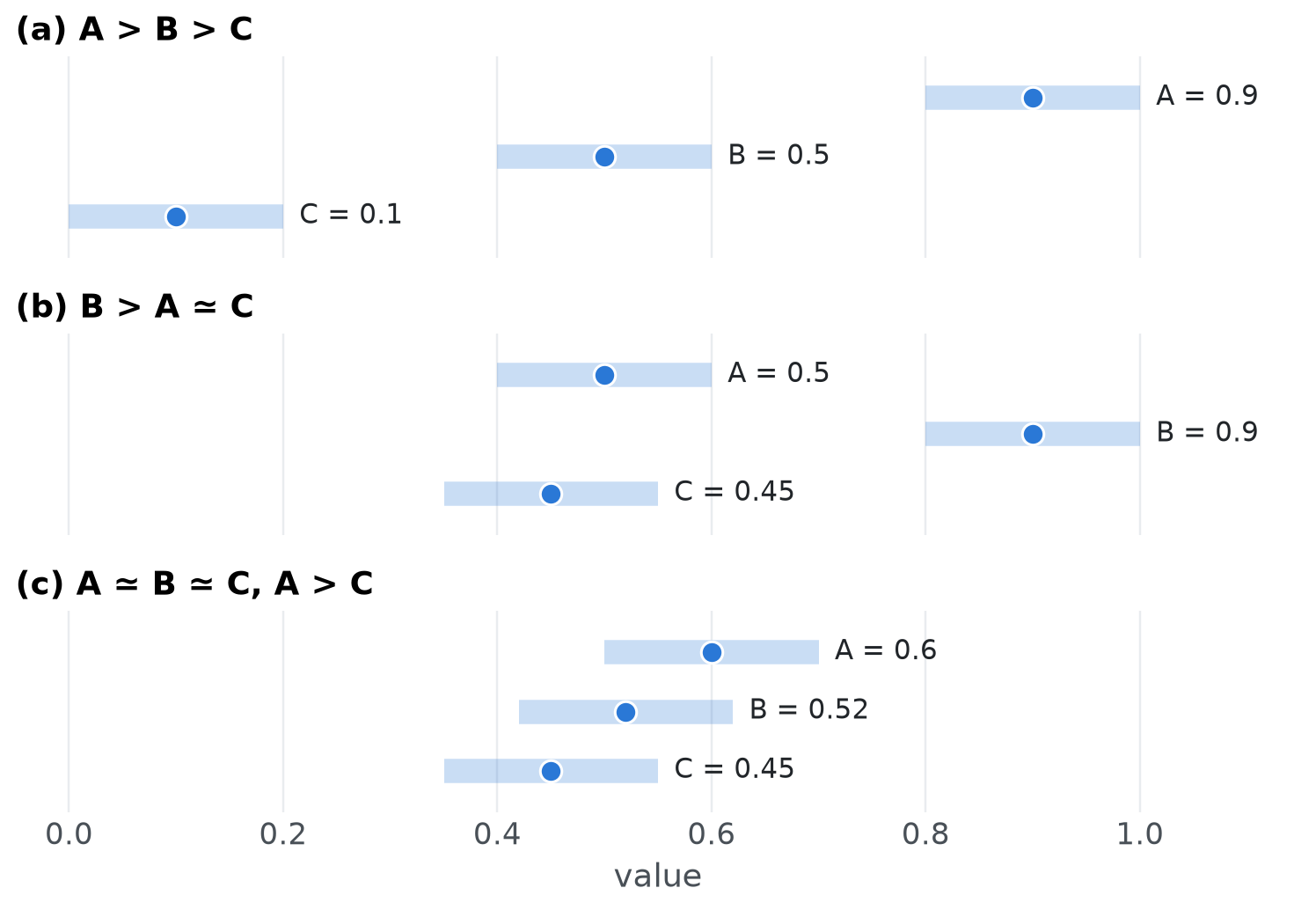
Here are results that give the three patterns of the figure above, with a threshold of 0.1. In the plot, the band around each value covers the values that are about the same as it, within the threshold: two stimuli are about the same when each lies in the other’s band.
examples = {
    "(a) A > B > C": [0.9, 0.5, 0.1],
    "(b) B > A ≃ C": [0.5, 0.9, 0.45],
    "(c) A ≃ B ≃ C, A > C": [0.6, 0.52, 0.45],
}
intervals(examples, T=0.1, name="examples")
for title, values in examples.items():
    print(title)
    print(clobe.imac(torch.tensor(values), (0.1, -0.1)), end="\n\n")
(a) A > B > C
tensor([[2., 1., 1.],
        [2., 2., 1.],
        [2., 2., 2.]])

(b) B > A ≃ C
tensor([[ 2., -1.,  0.],
        [ 2.,  2.,  1.],
        [ 2.,  2.,  2.]])

(c) A ≃ B ≃ C, A > C
tensor([[2., 0., 1.],
        [2., 2., 0.],
        [2., 2., 2.]])
Read it row against column, counting from 0. Row 0, column 1 is 1: stimulus 0 (0.9) is larger than stimulus 1 (0.5). Row 1, column 2 is 0: 0.5 and 0.45 are within 0.1 of each other. The diagonal and everything below it are set to 2, because they repeat information already in the upper triangle (the relation of \(j\) to \(i\) is the opposite of \(i\) to \(j\)). So a pattern over \(n\) stimuli consists of \(n(n-1)/2\) relations, one per pair.
Two results have the same pattern if their upper triangles are equal, even if their numbers differ:
a = clobe.imac(torch.tensor([0.9, 0.5, 0.45, 0.1]), (0.1, -0.1))
b = clobe.imac(torch.tensor([0.8, 0.4, 0.42, 0.2]), (0.1, -0.1))
torch.equal(upper(a), upper(b))
True
imac() works on a whole batch of results at once: a (n, k) tensor of results gives a (n, k, k) tensor of matrices. That is what lets it be the discretize of a psp.PSP run.
clobe.imac(torch.tensor([[0.9, 0.5, 0.45, 0.1], [0.8, 0.4, 0.42, 0.2]]), (0.1, -0.1)).shape
torch.Size([2, 4, 4])
A note on rounding#
Computers store most decimals inexactly: 0.3 - 0.2 is not quite 0.1.
0.3 - 0.2 == 0.1
False
Without care, a difference that should sit exactly on the threshold could land on either side of it depending on which numbers produced it. imac() compares differences with a tiny tolerance, clobe.TOLERANCE (about \(1.5 \times 10^{-8}\), as in the R package), so equal steps are always treated alike.
In float32, which is what makes a GPU worthwhile, numbers are stored far less precisely: 0.3 - 0.2 is off by about \(10^{-8}\) in float64 but by about \(10^{-7}\) in float32, more than the tolerance. For float32 and lower precision, imac() therefore uses a tolerance of 8 machine epsilons of the dtype instead, so that equal steps are still treated alike:
steps = torch.tensor([0.4, 0.3, 0.2, 0.1])  # float32
upper(clobe.imac(steps, (0.1, -0.1))), upper(clobe.imac(steps.double(), (0.1, -0.1)))
(tensor([0., 1., 1., 0., 1., 0.]),
 tensor([0., 1., 1., 0., 1., 0.], dtype=torch.float64))
Inclusive thresholds#
Versions of clobe before 0.8.0 counted a difference exactly equal to the threshold as larger (or smaller) rather than about the same, without a tolerance. inclusive=True gives that rule, for reproducing analyses made with them, such as the OSCAR routine (Dome & Wills, 2026) in psp.models.oscar:
values = torch.tensor([0.5, 0.25, 0.0], dtype=torch.float64)
upper(clobe.imac(values, (0.25, -0.25))), upper(clobe.imac(values, (0.25, -0.25), inclusive=True))
(tensor([0., 1., 0.], dtype=torch.float64),
 tensor([1., 1., 1.], dtype=torch.float64))
“About the same” is not transitive#
The relation “is larger than” behaves as you would expect: if \(a\) is larger than \(b\) and \(b\) is larger than \(c\), then \(a\) is larger than \(c\). “About the same” does not. Here is a classic illustration (Luce, 1956): you cannot taste the difference between a cup of coffee with 50 grains of sugar and one with 51, nor between 51 and 52, and so on, yet you can certainly taste the difference between 50 and 100 grains.
The same happens with any threshold:
clobe.imac(torch.tensor([0.50, 0.58, 0.66]), thresholds=(0.1, -0.1))
tensor([[ 2.,  0., -1.],
        [ 2.,  2.,  0.],
        [ 2.,  2.,  2.]])
intervals({"0.50, 0.58, 0.66 with a threshold of 0.1": [0.50, 0.58, 0.66]}, T=0.1, name="coffee")
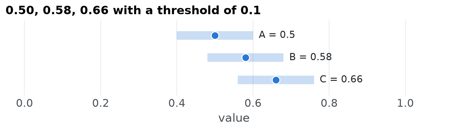
Stimuli 0 and 1 are about the same (they differ by 0.08), as are 1 and 2, but stimulus 0 is smaller than stimulus 2 (they differ by 0.16).
Semiorders#
A relation built this way, where \(a\) counts as larger than \(b\) only when it exceeds \(b\) by more than a fixed margin,
is called a semiorder (Luce, 1956). Scott and Suppes (1958) showed that, on a finite set, these are exactly the relations \(\succ\) with three properties:
Nothing is larger than itself.
If \(a \succ b\) and \(c \succ d\), then \(a \succ d\) or \(c \succ b\). (Two clear differences cannot “cross” each other.)
If \(a \succ b\) and \(b \succ c\), then for any other \(d\), \(a \succ d\) or \(d \succ c\). (A gap of two clear steps is too wide for anything to be about the same as both ends.)
So every inequality matrix from imac() with symmetric thresholds is a semiorder, and this is the default, ordering="semiorder". It is the right choice when the threshold expresses measurement uncertainty, as it usually does.
Weak orderings#
Sometimes we want “about the same” to mean “exactly tied”. Then the relation is a weak ordering: a ranking in which ties are allowed. Its tied groups can be ranked from top to bottom, and “tied with” is transitive. With ordering="weak", imac() ignores the thresholds and treats only exact ties as equal:
(clobe.imac(torch.tensor([0.50, 0.58, 0.66]), (0.1, -0.1), ordering="weak"),
 clobe.imac(torch.tensor([0.50, 0.50, 0.66]), (0.1, -0.1), ordering="weak"))
(tensor([[ 2., -1., -1.],
         [ 2.,  2., -1.],
         [ 2.,  2.,  2.]]),
 tensor([[ 2.,  0., -1.],
         [ 2.,  2., -1.],
         [ 2.,  2.,  2.]]))
Formally, a weak ordering is a semiorder with \(T = 0\): \(a \succ b \iff u(a) > u(b)\).
What the difference looks like#
Every weak ordering is a semiorder, but not the other way round. For three stimuli there are 19 semiorders and 13 weak orderings. The 6 extra patterns are exactly the “sugar in coffee” chains: two neighbours are each about the same as the middle stimulus but clearly different from each other, in each of the six ways of assigning stimuli to the three positions.
semi = clobe.orderings(3).inequality_matrices
weak = clobe.orderings(3, ordering="weak").inequality_matrices
weak_keys = {tuple(row.tolist()) for row in upper(weak)}
extra = semi[[tuple(row.tolist()) not in weak_keys for row in upper(semi)]]
len(extra), extra[0]
(6,
 tensor([[ 2, -1,  0],
         [ 2,  2,  0],
         [ 2,  2,  2]], dtype=torch.int8))
In this one, stimulus 2 is about the same as both 0 and 1, but 0 is smaller than 1. (orderings() returns its matrices as int8, which takes an eighth of the memory of float64; they compare equal to the float matrices of imac().)
Choosing the thresholds#
Use symmetric thresholds,
(T, -T). With asymmetric thresholds, whether a pair counts as different depends on which stimulus comes first, which is rarely intended.Choose \(T\) from how precisely the dependent variable is measured. For proportions from \(N\) trials, one trial is a step of \(1/N\).
The patterns you can observe also depend on how finely the measurement scale is divided relative to \(T\). universal-set.ipynb shows why this matters when counting the possible patterns.
References#
Dome, L., & Wills, A. J. (2025). g-Distance: On the comparison of model and human heterogeneity. Psychological Review, 132(3), 632-655. https://doi.org/10.1037/rev0000550
Dome, L., & Wills, A. J. (2026). Errorless Irrationality: A unified computational account of the inverse base-rate effect across predictive, observational, and unsupervised procedures (arXiv:2608.06149). arXiv. https://doi.org/10.48550/arXiv.2608.06149
Navarro, D. J., & Lee, M. D. (2005). An application of minimum description length clustering to partitioning learning curves. Proceedings of the 2005 IEEE International Symposium on Information Theory (pp. 587-591).
Pitt, M. A., Kim, W., Navarro, D. J., & Myung, J. I. (2006). Global model analysis by parameter space partitioning. Psychological Review, 113(1), 57-83. https://doi.org/10.1037/0033-295X.113.1.57
Luce, R. D. (1956). Semiorders and a theory of utility discrimination. Econometrica, 24(2), 178-191. https://doi.org/10.2307/1905751
Scott, D., & Suppes, P. (1958). Foundational aspects of theories of measurement. Journal of Symbolic Logic, 23(2), 113-128. https://doi.org/10.2307/2964389